Every Wardley mapper quickly learns the difference between graphs and maps: the space on a map has meaning, whereas space on a graph has none. Another way of framing this is that a Wardley Map is a Euclidean embedding (information is projected onto a Euclidean space, a vertical and horizontal axis). A graph is a non-Euclidean embedding (information content is in the vertices and edges and attributes of the graph).
Euclidean embedding is an excellent interface for people as it is optimized for human visual processing of information. For Wardley Map tool builders, the Euclidean embedding is typically represented in a machine as x and y coordinates. I intend to demonstrate below that a non-Euclidean Wardley Map embedding in a semantic spacetime (a Wardley Graph) seems to be a better machine representation for Wardley Maps tooling.
Semantic Spacetime
Mark Burgess explains the nature of semantic spacetime in his book: “Smart Spacetime: How Information Challenges our Ideas About Space, Time, and Process”, but the key inspiration for this post is his Universal Data Analytics as Semantic Spacetime series on Medium. Below, I very quickly summarize the portion relevant to understanding what follows.
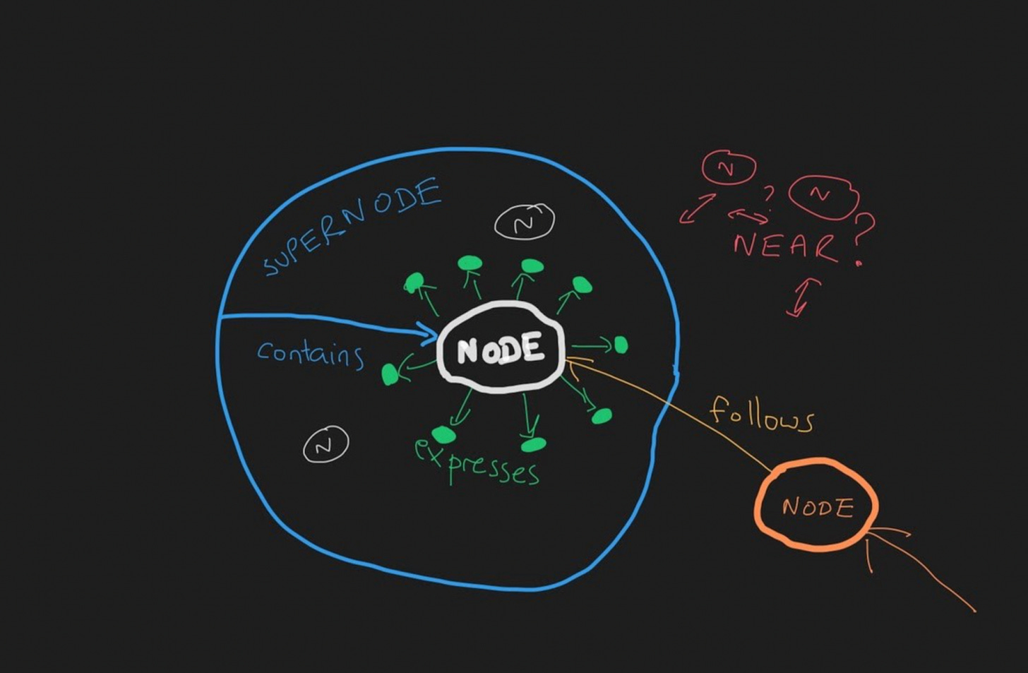
Within semantic spacetime, there exist four meta-types of semantic links, which describe process causal structure. That is, there are, fundamentally, only four kinds of relationships:
CONTAINS (where A contains B) - a container/space-like relationship; to be inside or outside (part of); math analogy is a polar vector
FOLLOWS (where A follows B) - a sequential/time-like relationship; to follow or precede; math analogy is a translation vector
EXPRESSES (where A expresses B) - a local property being expressed; to express information; math analogy is a scalar property
NEAR (where A is near B) - a similarity/nearness relationship; to be next to another location; math analogy is a primitive vector
Each one of the above types can be expressed in four directions:
Forward - e.g.: “Contains”
Backward - e.g.: “Is Contained By”
Negative-Forward - e.g.: “Does Not Contain”
Negative-Backward - e.g.: “Is Not Contained By”
A table description may be helpful:
And in an illustration form:
For specific instances of a link, we would add a specific type to the meta-type. For example: “Is Like” (NEAR), “After” (FOLLOWS), “Depends On” (FOLLOWS), etc.
Examples and intuition regarding specific types1:
With this understanding of semantic spacetime, how do we embed a Wardley Map in it?
The Vertical Axis
The information contained within a Wardley Map vertical axis traditionally represents the value chain. Relative position is the primary information content and is typically modeled by a dependency graph. The semantic link type of the dependencies between components in a value chain is "depends on" (FOLLOWS).
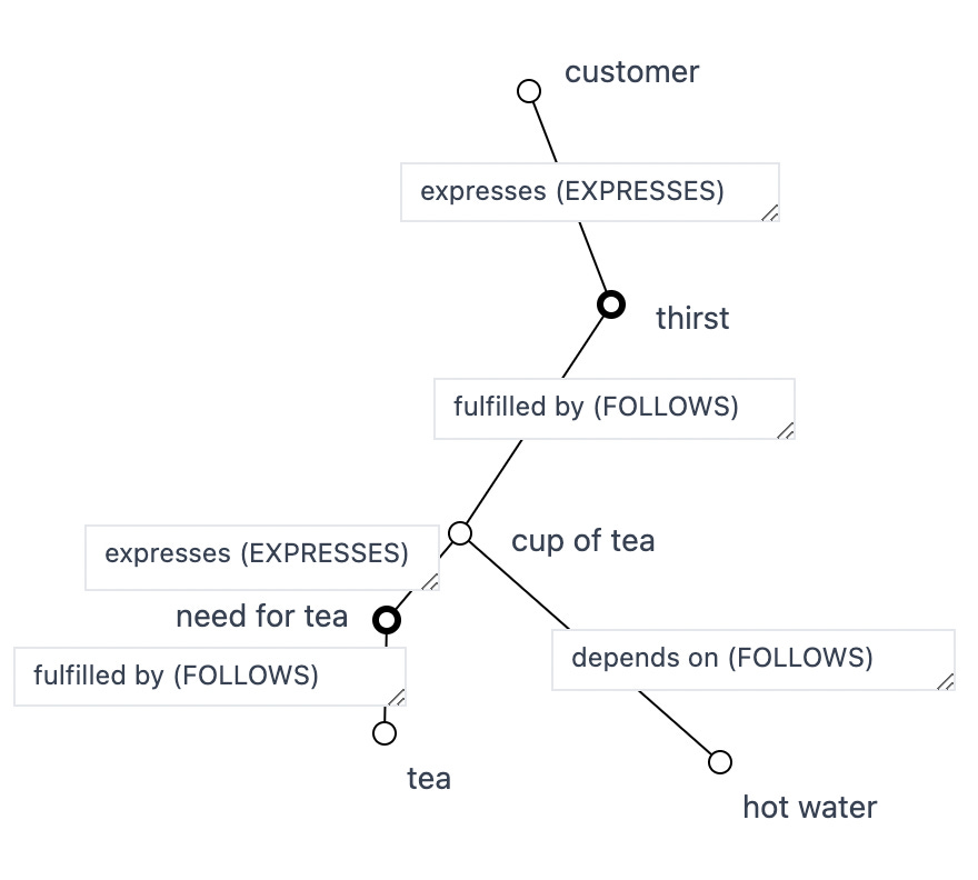
The semantics appear to change near the customer, as the customer expresses a user need (such as "thirst"). The semantic link type of the value chain dependency between a customer and the user need is "expresses" (EXPRESSES).
What then, is the elementary type of link between the user need and the component that fulfills that need? It is another type of FOLLOWS, specifically “fulfilled by” (FOLLOWS).
Visually:
Within the value stream context, it is of note that the customer/user need/offering is only modeled at the edge of the map near the customer anchor (expresses (EXPRESSES) + fulfilled by (FOLLOWS)) and not modeled in the dependency chain of the value stream (all of the “depends on” (FOLLOWS) links). If we consider what needs to happen for the cup of tea component to instantiate, we see that a cup of tea EXPRESSES the need for tea and hot water, and those have to be “fulfilled by” (FOLLOWS) the tea and hot water components.
From this, we can see that a “depends on” (FOLLOWS) link is an aggregate of a component “expressing” (EXPRESSES) a user need which is “fulfilled by” (FOLLOWS) an offering fulfilling the need. That is, if we “zoom in” on a “depends on” (FOLLOWS) link we observe a user need appear surrounded by “expressing” (EXPRESSES) and “fulfilled by” (FOLLOWS) links. For example, “zooming in” into the link between cup of tea and tea:
Again, we typically don’t “zoom in” like this on a map, but my intent here is to demonstrate a certain equivalence present between semantic links in the value chain once they are projected into semantic spacetime.
Just Scaffolding


Simon Wardley often points out that the vertical position on a Wardley Map is "just scaffolding". Having seen it now from the semantic spacetime framing, this may be due to all of the information being contained in the graph links, that is, the relative non-Euclidean position with respect to the other nodes. The Wardley Graph directly represents the Wardley Map value chain as nodes and edges.
Horizontal Axis
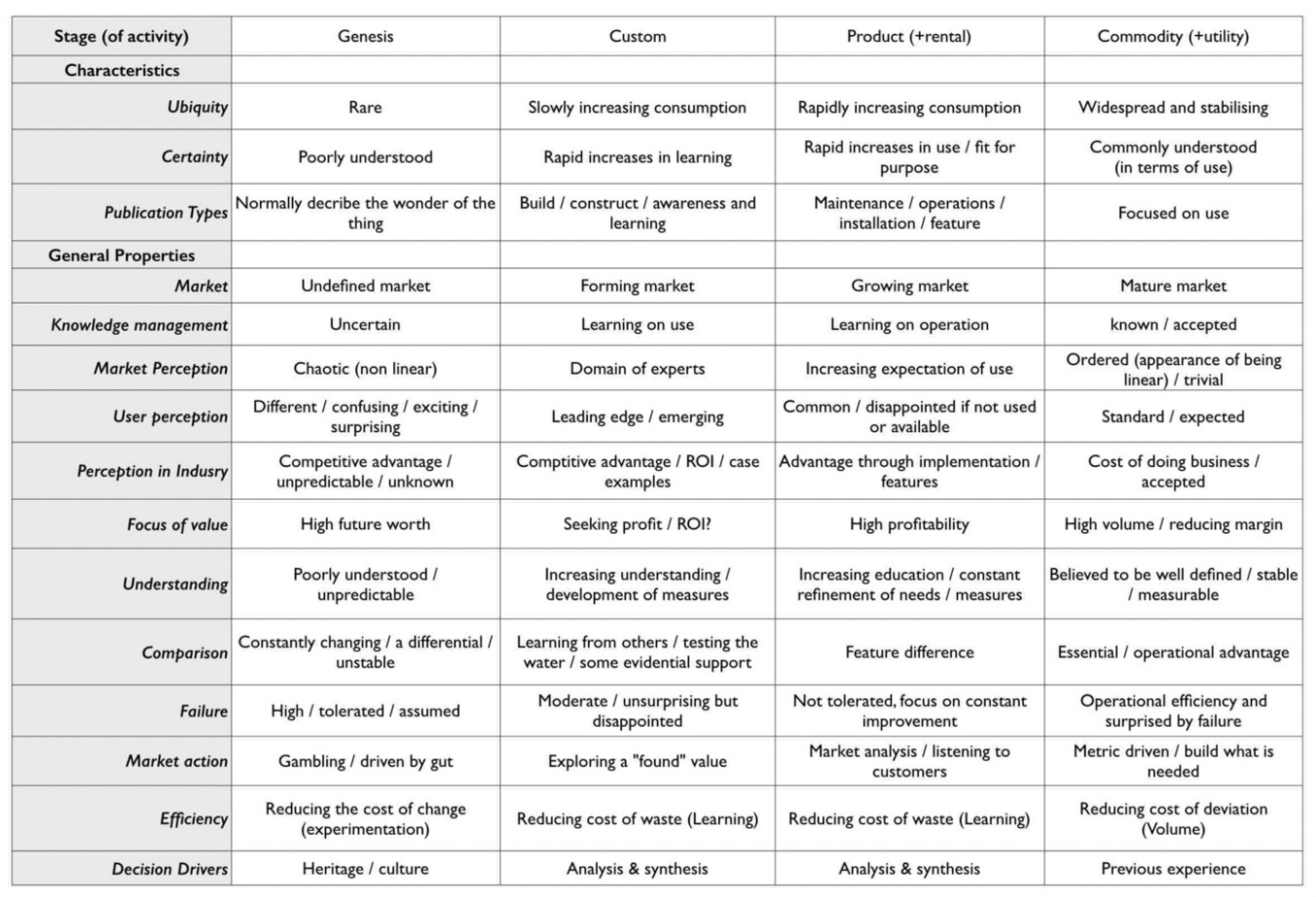
The horizontal-axis of a Wardley Map traditionally maps to the stages of evolution2. In order to determine the horizontal coordinate, the stages of evolution cheat sheet offers qualitative guidance:
For a machine, rather than storing an x coordinate between 0 and 1, it is more effective to retain the specific semantic links to each of the qualitative properties.
I explored machine encoding of the horizontal axis in https://mappingevolution.com, where I collected human (Euclidean projected) input in response to prompts for selecting how NEAR a component under consideration is to each characteristic of each evolutionary stage. This input was then interpreted as a four-dimensional vector with a weight assigned to each stage of evolution. The resultant four-dimensional vector was a summary of an underlying graph of relationships and allowed for aggregation across multiple summaries.
In order to retain the semantic spacetime graph, the approach here is to create a graph between the component and each characteristic in each evolutionary stage using EXPRESSES links. Visually, it looks something like this:
We can retain the meaning of a component being in the Product stage by having most of its links EXPRESS a characteristic that is CONTAINED by the Product stage. Similarly, a component with all links EXPRESSING characteristics CONTAINED by the Commodity stage would correspond to being a Commodity.
This graph representation retains the ability to aggregate multiple summaries by assigning weight to each EXPRESS link based on the count of its occurrences in the individual samples being aggregated.
Additional benefit is that there is no forcing of position in Euclidean space. If an EXPRESS link exists, it contributes to how much Product-ness is being EXPRESSED by the component. If the link does not exist, it has no effect.
This graph representation also enables a graph algorithm for summarizing an entire Wardley Map into a single component (described later).
Characteristics and General Properties Themselves
The characteristics and general properties of the stages of evolution themselves, instead of a table in the illustration above, can also be expressed as a graph. For example, the general property of Failure at each stage: tolerated, disappointed, not tolerated, surprised has bidirectional NEAR links between the stages:
tolerated is NEAR disappointed
disappointed is NEAR not tolerated
not tolerated is NEAR surprised
Notice that these are not transitive in the sense that Failure being tolerated is not NEAR being surprised by Failure. In general, Genesis is NEAR Custom, which is NEAR Product, which is NEAR Commodity.
Aside from the bidirectional NEAR links, there also exist unidirectional ("evolved from") FOLLOWS links:
disappointed FOLLOWS tolerated
not tolerated FOLLOWS disappointed
surprised FOLLOWS not tolerated
(and in the case of Obsolescence Climatic Pattern3)
not tolerated FOLLOWS surprised
disappointed FOLLOWS not tolerated
In general, Genesis is FOLLOWED by Custom, which is FOLLOWED by Product, which is FOLLOWED by Commodity, (and in the case of Obsolescence Climatic Pattern) which is FOLLOWED by Product, which is FOLLOWED by Custom.
In the context of Obsolescence Climatic Pattern, there are interesting differences in characteristics expressed by a component in Custom at the beginning of its existence when compared to being in Custom at the end of its existence.
Recovering the Horizontal Axis
The idea of the Wardley Graph is to maintain a graph machine representation for a Wardley Map. This means we need to be able to recover a Wardley Map from a Wardley Graph. For a demonstration, let’s consider the classic Cup of Tea map:
With the Cup of Tea map encoded as a Wardley Graph, we can project it onto Euclidean space, and we see something like this:
First, this is clearly not a Wardley Map. The idea here is to demonstrate that the essential information that we typically extract from the horizontal axis position is present in the graph links. The projection above is done using force-directed graph drawing. Notice the presence of stages of evolution I, II, III, and IV and imagine the horizontal axis aligned along that sequence of nodes. We see that where each component is located ends up corresponding to where it is present on the original Wardley Map. This means that the graph alone contains enough information to reconstruct the horizontal axis coordinate from the graph information alone.
Another thing of note is the location of the customers expressing user needs (Public and Thirst for Tea are highlighted in the picture). I often experience a lot of anxiety of where to place the customer on the evolutionary axis. Within the Wardley Mapping community, there are also methods that depict the customer using different horizontal labels, or even a completely different coordinate system like the user journey. The Wardley Graph encoding can demonstrate that customers and user needs are a boundary condition and do not need to be associated with stages of evolution to be useful.
Movement
Components Move
Throughout the stages of a component's evolution, the component updates the EXPRESSES links between itself and the various stages of each evolutionary characteristic. The aggregation of these links viewed at different times changes as the component EXPRESSES more characteristics CONTAINED by one stage of evolution vs another (Genesis, Custom, Product, or Commodity). When these snapshots are viewed over time, an effect corresponding to what we label as "movement" occurs.
This same movement occurs on the Wardley Graph:

If you’re having trouble seeing the similarity, consider this visualization showing the same movement as the videos above, but this time on a Wardley Graph with nodes arranged in the familiar grid pattern:
Moving Components
One of the uses of Wardley Maps is to determine what actions to take where on the map. One of those actions may be to accelerate a component along its evolutionary trajectory. In order to move a component in semantic spacetime towards a more desired state of evolution, we can evaluate each characteristic and focus on the component EXPRESSING a different characteristic through our actions in the world. For example, increasing components ubiquity by switching to mass manufacturing methods.
This framing highlights that some characteristics may be actionable/controllable/leading (switch from experimental investment to searching for profit), while others may be unactionable/lagging (user perception, market perception).
Jabe Bloom (@cyetain) points out that "movement is not free", therefore, affecting component characteristics requires action that expends time and treasure. Chris Daniel (@wardleymaps) points out that some moves are too expensive to make: "toxic legacy", therefore, some changes in characteristics may be completely out of reach.
Summary/Aggregation
So, we have a Wardley Graph, what is the benefit?
One of the problems that machines need to deal with that humans do automatically is summary and aggregation of components on Wardley Maps. On the Cup of Tea map there is a Power component. This is fairly abstract, but if needed, we could replace the Power component with wall socket, breakers, panels, wires, power stations, etc. In machine representation, we need to be able to do something similar, and this is where Wardley Graph machine representation is really useful.
Instead of saying this is possible in the abstract, we can instead define a graph algorithm for Wardley Map component summary based on Mark Burgess’ algorithm for grouping nodes into supernodes4. The algorithm below is written in terms of summarizing all map components (excluding user needs and customers), but works just the same for summarizing only a subset of map components.
Map components are all marked under a single "hub" component (the summary component for the map). All the map components are linked to the hub with a CONTAINS link, specifically "Is contained by" (CONTAINS).
Aggregate information about each map component is aggregated into the hub component. This information is:
Total count of map components (aggregated from existing counts if map consists of hub components already).
Any other scalar-like property of the nodes, ex: EXPRESS links summed up and tallied
Consider other graph machine learning node features. For example, a Graphlet Degree Vector (GDV) could express the particular way that components express evolutionary characteristics. The specific graphlet count could indicate how many characteristics are expressed by the component.
Links from summarized components to things that are outside of the hub are copied to the hub component. Repeated links are summed and represented as link weight.
For information encoded in the vertical axis (value chain), the hub component does not include user needs and customers, those remain outside of the hub.
For information encoded in the horizontal axis (evolution), all of the component EXPRESS links designating their stage of evolution are aggregated and summed as link weights at the hub level, thus determining the hub's summary stage of evolution.
As a result of the above algorithm, the hub becomes a single component, ready to answer queries, and can be used as a component of another map, thus expressing the fractal nature of Wardley Map components. For example, the above algorithm can generate a summary Tea Shop component for the entire Cup of Tea map. Note in the illustration below that the Tea Shop ends up projecting into space where you’d expect it to. Also note that the summary of Tea Shop (without Kettle) is also where you’d expect it to be.
With the Tea Shop, we have an example of summarizing many components into a single summary component. Another use for the summary algorithm is to integrate multiple points of view of the same component, a version of crowdsourcing. Multiple people (and machines) can determine characteristics expressed by some component. The summary algorithm can then integrate all those points of view and provide a crowdsourced version of the component. This is another powerful collaboration feature enabled by the Wardley Graph.
Another benefit of automated summary are component updates. When a constituent component is updated, the summary and anything else connected can be updated automatically as well.
What is a Map?
How should maps be represented on the Wardley Graph?
I think it is worth making the distinction between a map and a component that summarizes other components. That is, a map is not a summary component. A map does not contain other maps. A map simply contains the components, customers, and user needs that are depicted on the map:
Another, example of a smaller map containing fewer components:
As mentioned before, a map is not the same as a summary component. Here is an example of a map that contains the Tea Shop summary component as part of the map:
With maps and components being distinct from each other we end up with a representation where maps can have both, the summary component and at the same time highlight some of that component’s constituents. For example, the kettle situation in the Tea Shop:
What’s Next?
The above is what I’ve been able to put together so far in my exploration of embedding Wardley Maps in non-Euclidean semantic spacetime. I hope you enjoyed the journey and see Wardley Maps from a new perspective. I very much recognize the irony of promoting a graph to represent a map, but I hope I made the context clear for when to use a graph (machine representation) and when to use a map (human interface).
As a tool builder, I find this graph representation very compelling and sympathetic to the problems I encountered when attempting to create a useful machine representation. I hope that by sharing it with you we can improve the capabilities of our tools and perhaps this could become a useful common foundation for a common interface/representation between our various systems.
To learn more about semantic spacetime and the underlying foundation for the whole graph thing I recommend Mark Burgess’ series: Universal Data Analytics as Semantic Spacetime. After going through Marks’ material, I adapted his SST library (https://github.com/markburgess/SemanticSpaceTime) into a format more familiar to me, resulting in my version of the sst library (https://github.com/tristanls/sst). These establish the semantic spacetime foundation on which Wardley Graph is built.
For the Wardley Graph implementation itself, my experimental library is https://github.com/tristanls/wardleygraph, where you can see semantic spacetime concepts adapted specifically for the Wardley Graph use case. Additionally, that’s where you’ll find reference implementation of the summary algorithm and examples of how to encode the information contained in a Wardley Map into a graph.
There is plenty more to do and learn. Graph machine learning comes to mind. What would scenario planning look like on a Wardley Graph? Can I subscribe to components maintained by experts? Does a graph make it easier? The current implementation uses ArangoDB as the graph database, I intend to explore using Amazon Neptune next. I hope you find the graph representation as compelling as I do, and I look forward to seeing what the Wardley Mapping community can do with it.
Burgess, Mark. Smart Spacetime: How information challenges our ideas about space, time, and process (Kindle Location 6668). Kindle Edition.
Wardley, Simon. Wardley Mapping Book, Chapter 2: Finding a Path, accessed on 4 Jan 2022.
Slominski, Tristan. Obsolescence Climactic[sic] Pattern: When Things Move to the Left, accessed on 4 Jan 2022.
Burgess, Mark. Respecting the graph directly, accessed on 4 Jan 2022.


